Applying Transformation

In order to find a proper transformation between two consequent frames several approaches can be used. For example, the so-called SIFT (Scale-Invariant Feature Transform) algorithm finds multiple distinctive invariant features on each frame, so that these features can be used to perform reliable matching between the subsequent frames. For this particular application, featuring a very distinctive texture, the SIFT algorithm exhibits a very good performance finding around 160 keypoints on each frame. Around a half of them find the correct match with the keypoints on the following frame. For example, for the two images shown in Fig.B (one corresponds to the instant of time preceding the pop-up event and another one has a new popped-up point) 76 matches are found. Rough averaging between all matches resulteds in a 0.547° rotation angle.

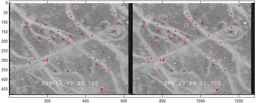
              Figure B. Multiple matching points of the SIFT algorithm.

The matching pairs of points found with the SIFT algorithm or somehow else (hereinafter called control points) can be further used to infer a more general, spatial transformation or an inverse mapping from the output space (x,y) to input space (u,v) according to the chosen transform type. There are several transform types that can be used for the specific application in order to find a better match between the two images. The first three, requiring lesser control-point pairs are the linear conformal, affine and projective transformations

• Linear conformal – assumes that shapes in the input image are unchanged, but the image is distorted by some combination of translation, rotation, and scaling, i.e. the straight lines remain straight, and parallel lines are still parallel

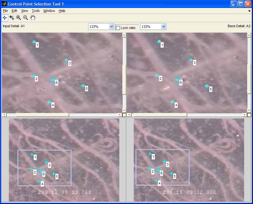
The following presents an example of using the multiple pairs of control points assigned manually using the MATLAB Control Point Selection Tool. When being called, the Control Point Selection Tool allows assigning multiple pairs of the control points either manually (as shown in Fig.C) or in the prompt regime (available after assigning at least two points manually), when the potential matches are predicted manually (as shown in Fig.D).

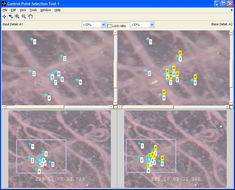Figure C. Picking the pairs of control points manually.	Figure D. Picking the pairs of control points semi-automatically.

When the appropriate number of points is assigned, the algorithm continues with their correction (based on cross correlation) and computation of the corresponding transformation. Figure E presents an example, when the linear conformal transformation was used to correct the input image (shown on the top right). The corrected image (bottom right) reveals the parameters of transformation (note, all images are cropped by 10 pixels from the left, up and bottom and by 20 pixels from the right to eliminate the black selvage).

Shown on the bottom left is the raw difference between the base and input (uncorrected) frames. Supposedly, if applied to the corrected image it should only reveal the popped-up objects (in this case their position within the image frame could be extracted very easily). Figure F presents this corrected difference for the linear conformal transformation. It is clearly seen that the picture appears cleaner as compared to the bottom left plot in Fig.E. The average intensity drops from 3.73 in Fig.E to 1.47 in Fig.F. However, Fig.F still shows some remnants of the texture suggesting that affine or even projective transformation might be a better choice.

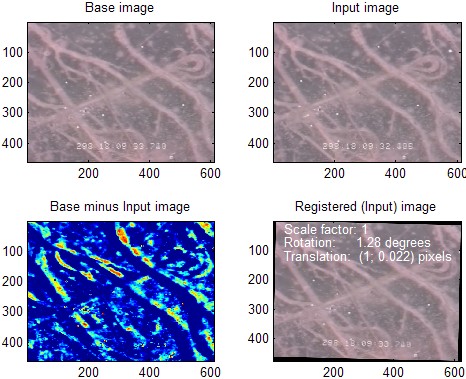
               Figure E. Applying the correction to the input image.

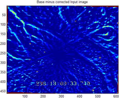
               Figure F. Difference between the base and corrected input image.

Nevertheless, it is clear that if something new pops up it should be much easier to detect it. Another useful outcome of correcting the frames, so that they reveal the same orientation as the base frame, meaning that the effect of motion of observer (aerial platform) is eliminated. In this case, playing the corrected frame sequence produces a “stabilized” video, so that all surveyed reference points remain at the same spots. It also helps blending EO and IR data (the IR images need to undergo the same preprocessing).

Since release 2013a MATLAB features several feature detection functions that may be used besides SIFT. These functions belong to the Computer Vision System Toolbox.